Financial Markets

I recently the online course Financial Markets, an introductory course about finance, and I was curious about how much knowledge there I could apply to programming.

Tools

I did everything in a Jupyter notebook then copies things over to this blog form. All the code samples were ran in python3.9, with these imports.

import numpy as np
from collections import defaultdict
from random import shuffle
from matplotlib import pyplot as plt 

Disclaimer

This post is not financial advice. I am not qualified to give financial advice. This post isn’t even meant to be useful in helping anyone financially: it’s just meant as a fun programming exercise.

The Cauchy Distribution

The basic format of this blog will be (1) create a function to simulate some investment strategy and (2) look at some statistics of it. This runs head-first into a really important fact about the markets: they’re prone to outliers.

To take my point here’s a running average of one million samples of the normal distribution:

total = 0
count = 0
points = []
least, most = 0, 0
for i in range(1000000):
    p = np.random.normal()
    least = min(least, p)
    most = max(most, p)
    total += p
    count += 1
    points.append(total / count)
print(least, most)
plt.plot(points)

-4.784901961310616 4.977789671795711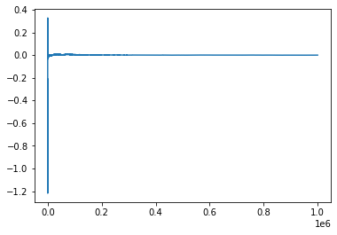

Because the number of samples is so large, as we average things out we very quickly go to zero. That shouldn’t be much of a surprise.

Here’s the same test, but replace np.random.normal with np.random.standard_cauchy:

-5137430.0782254785 192835.36382001732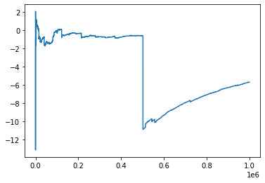

This is more in line with what the randomness of markets looks like. Events that would be basically impossible in a normal world are common on this distribution. In fact, extreme events are so common a lot of mathematical tools break down. For instance, Cauchy doesn’t have a mean.

As shown by the graph, Cauchy also doesn’t abide by the strong form of the Law of Large Numbers, which says you can average a bunch of samples of a distribution to get its mean. That makes it useless for finding statistics of distributions derived from it, so we have to ignore this fact and use normal instead.

Diversification

You’re financial portfolio should be diverse. Why? The risks average out.

Let’s try this by investing in 100 S&P500’s, which tends to average year-on-year returns of 10% with a 15 percent standard deviation.

def sp500():
    return 1.1 + np.random.normal() * 0.15

def portfolio1():
    return sum([ sp500() / 100 for _ in range(100) ])

We’ll re-use the following function to figure out how our hypothetical portfolio would perform:

def stats(f, samples_count=1000):
    samples = []
    for i in range(samples_count):
        samples.append(f())
    avg = np.average(samples)
    std = np.std(samples)
    print("Average: %.3f" % avg)
    print("Standard Deviation: %.3f" % std)
    print("95%% Confidence: %.3f - %.3f" % ((avg - 2 * std), (avg + 2 * std)) )

states(portfolio1)

Average: 1.100
Standard Deviation: 0.014
95% Confidence: 1.071 - 1.129

The result is we have exactly the same mean (a 10% return), but a much smaller standard deviation. The exact standard deviation is given by the variance sum law, but the point to know is all the randomness cancels out. In effect, we basically have a 10% risk-free rate of return. If we were able to leverage this bet, the return could be greater.

There’s a catch, though: in the real world there’s only one S&P500. The S&P500 is already the combination of a bunch of bets, most with much higher standard deviations of return, so we need to look for bets outside the market. Unfortunately pretty much anything we bet on is going to be heavily correlated with the S&P500.

According to CAPM a fully diversified portfolio is all we need. Once we have that we can just leverage up and down, and it’s impossible to do better.

Time

There’s another trick we can use to reduce our standard deviation of return: spin the wheel of time.

Here’s another portfolio where we simulate putting money into the S&P500, and keep it there for 100 years. Returns get reinvested.

def portfolio2():
    balance = 1
    for _ in range(100):
        balance *= sp500()
    return balance
stats(portfolio2)

Average: 12025.869
Standard Deviation: 21059.272
95% Confidence: -30092.675 - 54144.413

The result is large due to the effect of compound interest. Our investment grows by twelve thousand times (the actual average, 1.1 ** 100 is about 14 thousand). This twelve thousand times is the yield after 100 years, whereas 1.1 times is the annual yield. We can adjust back the annual yield by solving hundred_years_yield = X ** 100.

def portfolio3():
    balance = 1
    for _ in range(100):
        balance *= 1.1 + np.random.normal() * 0.15
    return np.power(balance, 1 / 100)
stats(portfolio3)

Average: 1.089
Standard Deviation: 0.015
95% Confidence: 1.059 - 1.120

I’m not sure why the average there is so far off from 1.1 (numerical accuracy?), but the important point is our standard deviation, previously 0.15 is now 0.015. Unlike before this doesn’t have a catch. We can make risky investments safer if we’re just willing to put it there for a long time.